Methodology: How to Develop a Trading Algorithm Honestly — a Reference Run

What this document is: not a new backtest result, but the methodology behind it. It describes the five-phase development workflow and uses the complete run of the paper series (DAX/FTSE/NQ/Dow, 2018–2026, net of spread) as a running example. No trading recommendation.

Most "profitable strategies" online are overfit. They look great on one market in one period and fail live. This document describes a workflow designed to prevent exactly that — through a sequence of hurdles every strategy must survive before real money comes into reach. The core is not a technique but an attitude: build the work so it can disprove itself.

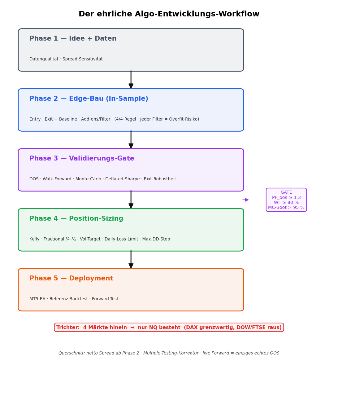
The three guiding principles

Before the phases: three rules that run across everything.

1. The funnel narrows. Every phase throws candidates out, never in. Whatever is carried into validation is a "trial" — and each extra trial raises the chance that something passes by luck. A few well-justified hypotheses beat many optimised ones.
2. Costs from Phase 2, not at the end. Spread (and later slippage) belongs in every R figure as soon as you optimise — not as a cosmetic correction at the close. A strategy that only works gross does not work.
3. Live forward is the only true out-of-sample. Every historical OOS block comes from the same dataset and is therefore never fully foreign. The honest final test only runs from today.

Phase 1 — Idea & Data

First make the idea mechanical (here: breakout of the 2nd 15-min candle after cash open) and present the data honestly before optimising anything: source, period, gaps, and a spread sensitivity — how much of the gross edge survives realistic costs? Overclaim here and you build on sand. → Example: 2nd opening candle

Phase 2 — Edge construction (all in-sample)

This is where the edge is built — in this order:

• Entry logic — the trigger.
• Exit logic + baseline — stop, break-even, trailing, take-profit. First define a baseline, then measure every modification against it. Finding in the example: only time break-even pays; trailing/partials/multi-TP cost expectancy.
• Add-ons / filters — pre-trade filters (NR4, bias, inside-day…) and in-trade add-ons (pyramiding). Right here, not later.

Every filter, every add-on is an extra parameter — and thus an overfit risk. The hurdle: an add-on must work across all tested markets (4/4 rule), otherwise it is curve-fit. In the example, of seven filters only the short bias generalised; pyramiding lowered Kelly growth at every size (the growth-optimal add size was 0). Both were honestly rejected. → Example: exit logic & add-ons

A key tool for add-ons: judge them not by profit factor but by the Kelly criterion (geometric growth) — it penalises variance and drawdown automatically and answers the right question: does the add-on make the strategy more growth- and more leverageable — or merely nominally bigger?

Phase 3 — The validation gate

The ruleset is fixed from here. Now one question only: does the edge survive on data that did not contribute to the selection? Four independent methods:

• Out-of-sample — in-sample selection, out-of-sample test on locked data.
• Walk-forward — rolling (sliding windows) and anchored (expanding): is the edge stable over time?
• Monte-Carlo — shuffle (drawdown distribution) and bootstrap (true probability of profit; a shuffle alone always gives P=100%).
• Deflated Sharpe — correction for the number of trials (multiple testing).
• Exit robustness — does the edge survive under structurally different exits? Then it lives in the entry, not in one exit mechanic.

The strict gate: PF_oos ≥ 1.3 and ≥ 80% profitable WF windows and recovery ≥ 2 and bootstrap P > 95%. In the example, of four indices — all of which looked identical in-sample (PF ~1.50) — only NQ passed every criterion; DAX borderline, DOW/FTSE failed. That is the whole point of the gate: the in-sample PF lies. → Example: validation gate

Phase 4 — Position sizing

Only after passing the gate may risk be discussed — and only on the core that passed. Tools: Kelly (optimal-f via maximising E[log(1+f·r)]), fractional Kelly (¼–½, because full Kelly is practically suicide), vol-targeting and hard risk overlays (daily-loss-limit, max-DD-stop). → Example: position sizing & Kelly

Phase 5 — Deployment & reality test

The finished system as a runnable MQL5 EA, then the real MT5 run against the most honest yardstick — buy-and-hold of the index. In the example NQ beats buy-and-hold ~2.1× (+273% vs +127% at the same drawdown), but real costs cost −72% return and triple the drawdown vs the idealised backtest. DAX real −1% → dead.

And the most uncomfortable lesson of the whole series — edge perishability: the real NQ run was strong through end-2024, then negative (2025 −9%, 2026 −11%) — while the backtest stayed green and it was not the costs. A backtest can lie, even a clean one. Only the live/forward test tells the truth; mechanical operation needs a rolling PF kill-switch, a discretionary overlay — or the discipline to retire a spent edge. → Example: MT5 algo & edge decay

From finding to algorithm: how to incorporate features

A discovered feature (e.g. "gap up → short is better", see 2nd candle) is not yet a rule. There are four common ways to turn such a finding into an algorithm — from overfit-prone to robust:

1. Hard filter (on/off): take the trade only if the condition holds. Simple — but every condition and every threshold is a parameter, it discards trades, and the cliff effect (just below excluded, just above included) is unrealistic.
2. Directional bias: the feature picks the side, not the whether (e.g. on a gap up, trade only the short side).
3. Conviction sizing (risk/size adjustment): all trades stay, but the position size scales with the expected edge — strong setups full risk, weak ones less, negative ones zero.
4. Score/model: combine several features into one score (logit/gradient-boosting → P(win) or expected R), then trade/size by it. Powerful, but the highest overfit risk.

Rule of thumb: way 3 (risk/size adjustment) is frequently the most robust. It needs no hard cutoff, uses a weak signal gradually rather than abruptly, and does not hinge on a single fitted threshold. Hard filters (way 1) often look better in the backtest but are the most prone to exactly the self-deception this methodology is built to prevent.

Discipline (the same for all four ways): selection ≠ validation (the feature must survive the gate on a separate block); count the trial count in the deflated Sharpe; few, cross-asset-consistent features (4/4 rule); continuous beats binary; and correlated features are not an additive edge (example: "close above ONR" and "gap up" both measure morning strength — stacking them does not double the advantage).

Worked through: conviction sizing on "short morning strength" (OOS)

So this isn't just theory, here is the concrete test of way 3. Three tiers from the robust findings of the 2nd-candle study: strong (short + morning strength), avoid (long against morning weakness), neutral. The tier weights are derived only from in-sample (≤ 2022), mean-normalised (same average exposure as flat → no hidden leverage) and applied out-of-sample (2023–2026). Pooled across all four indices:

OOS sizing	Total-R	meanR	Sharpe
Flat (1×)	253	0.075	1.39
Conviction	289	0.086	1.36

Finding: the sizing correctly reallocates toward the higher-expectancy shorts → +14% total-R — but no Sharpe gain (1.39 → 1.36); the extra return came with proportionally more variance. Mixed per index (DOW better, NQ/DAX slightly worse Sharpe, FTSE stays negative).

The real lesson: conviction sizing is the right, cliff-free way to use a signal — but it conjures no edge that isn't robustly there. A weak, partly correlated signal stays weak, however elegantly you size it. Had you looked only in-sample, you'd have booked the +14% total-R as "success" — the OOS test shows that risk-adjusted nothing was gained. Discipline beats technique.

The reference run in one table

What the five phases made of four candidates:

Market	In-sample PF	Phase-3 gate	Phase-5 role
NQ	~1.50	✅ passed	core algo
DAX	~1.50	❌ borderline	secondary, labelled
DOW	~1.50	❌ (PF)	rejected
FTSE	~1.50	❌ clearly	rejected

Four markets looked identical in-sample. The workflow filtered out three of them — that is the value of the methodology, not a single metric.

Checklist / decision gates

• Phase 1: idea mechanical? data honest? spread sensitivity computed?
• Phase 2: baseline defined? every modification measured against it? add-ons checked on 4/4, net of spread?
• Phase 3: ruleset fixed? OOS + WF + MC + DSR + robustness? gate criteria hard-defined before looking at the result?
• Phase 4: only on the gate-passing core? fractional instead of full Kelly? risk overlays?
• Phase 5: code = backtest logic 1:1? forward test set up?

Limitations of the methodology itself

This workflow is no guarantee either. The OOS block comes from the same dataset; the gate thresholds (1.3 / 80% / 95%) are justified but chosen values; the deflated Sharpe is assumption-sensitive; and the final truth comes only from live operation. The methodology minimises the risk of self-deception — it does not eliminate it.

---

📄 Full methodology as PDF · The series: Phase 1 · Phase 2 · Phase 3 · Phase 4 · Phase 5

Disclaimer: Historical statistics are no guarantee of future market behaviour. Not investment advice. Trading involves risk of loss up to total loss.