The Turn-of-the-Month Effect: a mechanism edge through the validation gate
Data basis: DAX / FTSE / NQ / Dow, daily cash close-to-close returns, Jan 2018 – Jun 2026, ~2,165 trading days / 101 month boundaries per index. Net of costs (2 pts round-trip per monthly trade). Not trading advice, no return promise.
The breakout series hunted for edges in the price — and mostly found noise. This study reverses the direction. It starts not from a pattern but from a mechanism: a reason why someone must trade at a specific time, regardless of price. That is where the most durable inefficiencies arise — because a non-profit-seeking participant is forced to act.
Around the month boundary, two such constraints collide. And the central lesson up front: a 'why' does not exempt you from the statistics. Even a well-reasoned mechanism must pass exactly the same validation gate as a blind price pattern.
The hypothesis: two forced mechanisms
(A) Inflow mechanism. Salaries, pension contributions, savings plans and dividend reinvestments arrive in a bundle around the first of the month and are deployed into the market largely regardless of price. → Expectation: an unconditional positive drift in the turn-of-month (TOM) window.
(B) Rebalancing mechanism. 60/40 and risk-parity funds must return to their target weights at month-end. After a strong equity month they are overweight → they sell equities; after a weak month → they buy. → Expectation: a conditional, mean-reverting effect — TOM weaker after up months, stronger after down months.
That makes the test interesting: (A) produces momentum-like drift, (B) the opposite. Which force dominates — and whether anything measurable survives at all — is decided by the test, not by the story.
Method: event study instead of candle scan
Identical discipline to the breakout series, only the tool is an event study:
- TOM window = last trading day of month M + first 3 trading days of M+1 (the classic Lakonishok-Smidt definition). That is ~19% of all trading days.
- Cross-asset (4/4): a mechanism edge must hold on several markets.
- In-sample (≤2022) → out-of-sample (≥2023).
- Net of costs in every number.
- Significance properly specified: Welch t-test of TOM vs. rest-of-month daily returns, plus an aggregate block bootstrap and a t-stat on the ~100 monthly trades.
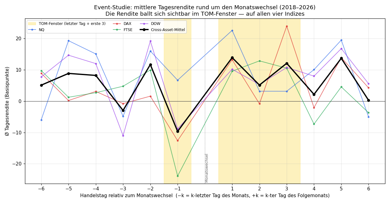
The average daily return clusters visibly in the TOM window (yellow) — on all four indices. But the picture is noisy. That is precisely the point of the whole study.
Finding 1 — the concentration (4/4)
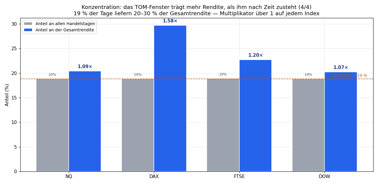
At first glance a clear hit: the TOM window carries more return than its time-share warrants on all four indices.
| Index | TOM days | TOM return share | Concentration | TOM avg/day | Rest avg/day |
|---|---|---|---|---|---|
| NQ | 18.8% | 20.4% | 1.09× | +8.9 bp | +8.0 bp |
| DAX | 18.8% | 29.7% | 1.58× | +6.0 bp | +3.3 bp |
| FTSE | 18.9% | 22.7% | 1.20× | +2.3 bp | +1.8 bp |
| Dow | 18.8% | 20.2% | 1.07× | +4.4 bp | +4.0 bp |
19% of days deliver 20–30% of total return. This is the number that ends up in marketing decks.
Finding 2 — the honest test (and the collapse)
Now the question that decides real vs. apparent: is the daily return difference between TOM and the rest of the month larger than the noise? Answer: no, nowhere.
| Index | TOM−Rest (diff) | Welch t | Trade t-stat | Verdict |
|---|---|---|---|---|
| NQ | +0.88 bp | +0.11 | +1.22 | not significant |
| DAX | +2.69 bp | +0.40 | +0.79 | not significant |
| FTSE | +0.47 bp | +0.09 | +0.28 | not significant |
| Dow | +0.37 bp | +0.06 | +0.67 | not significant |
| Pooled (4) | +1.10 bp | +0.33 | — | not significant |
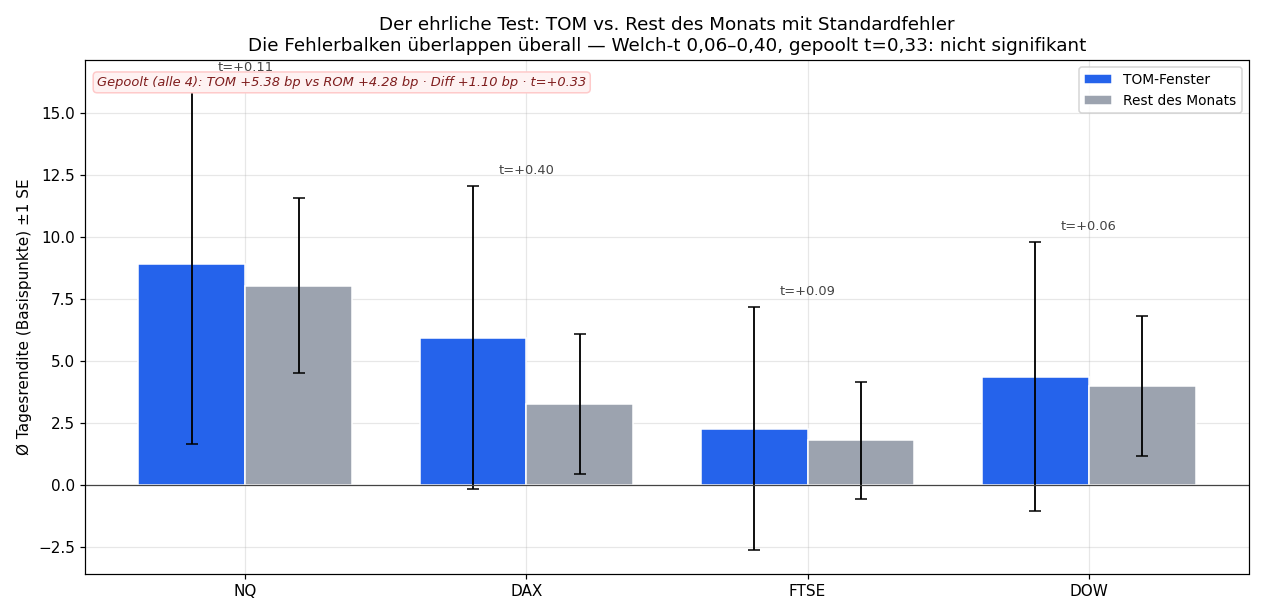
Even pooled across all four indices (n = 1,632 TOM days vs. 7,036 rest days) the t-value is 0.33 — worlds away from the 1.64 threshold. The error bars overlap massively.
How does that square with the 1.58× concentration? The concentration measures the cumulative return over 100 months — dominated by the market's general upward drift. The per-day effect, however, is only ~1–3 basis points, while daily volatility runs ~100–120 bp. A small systematic shift compounds over years into a pretty percentage — and remains statistically invisible all the same. This is exactly where most people fool themselves: an impressive aggregate statistic is not proof of significance.
Finding 3 — does it beat buy & hold?
The pragmatic counter-test: a strategy that is long only during the TOM window (19% of the time) and flat otherwise.
| Index | TOM-only CAGR | MaxDD | Sharpe | B&H CAGR | MaxDD | Sharpe |
|---|---|---|---|---|---|---|
| NQ | +3.6% | −15.5% | 0.40 | +19.6% | −35.6% | 0.88 |
| DAX | +2.3% | −14.3% | 0.31 | +8.0% | −38.3% | 0.50 |
| FTSE | +0.5% | −18.9% | 0.11 | +3.6% | −37.1% | 0.31 |
| Dow | +1.7% | −10.3% | 0.26 | +8.9% | −37.1% | 0.55 |
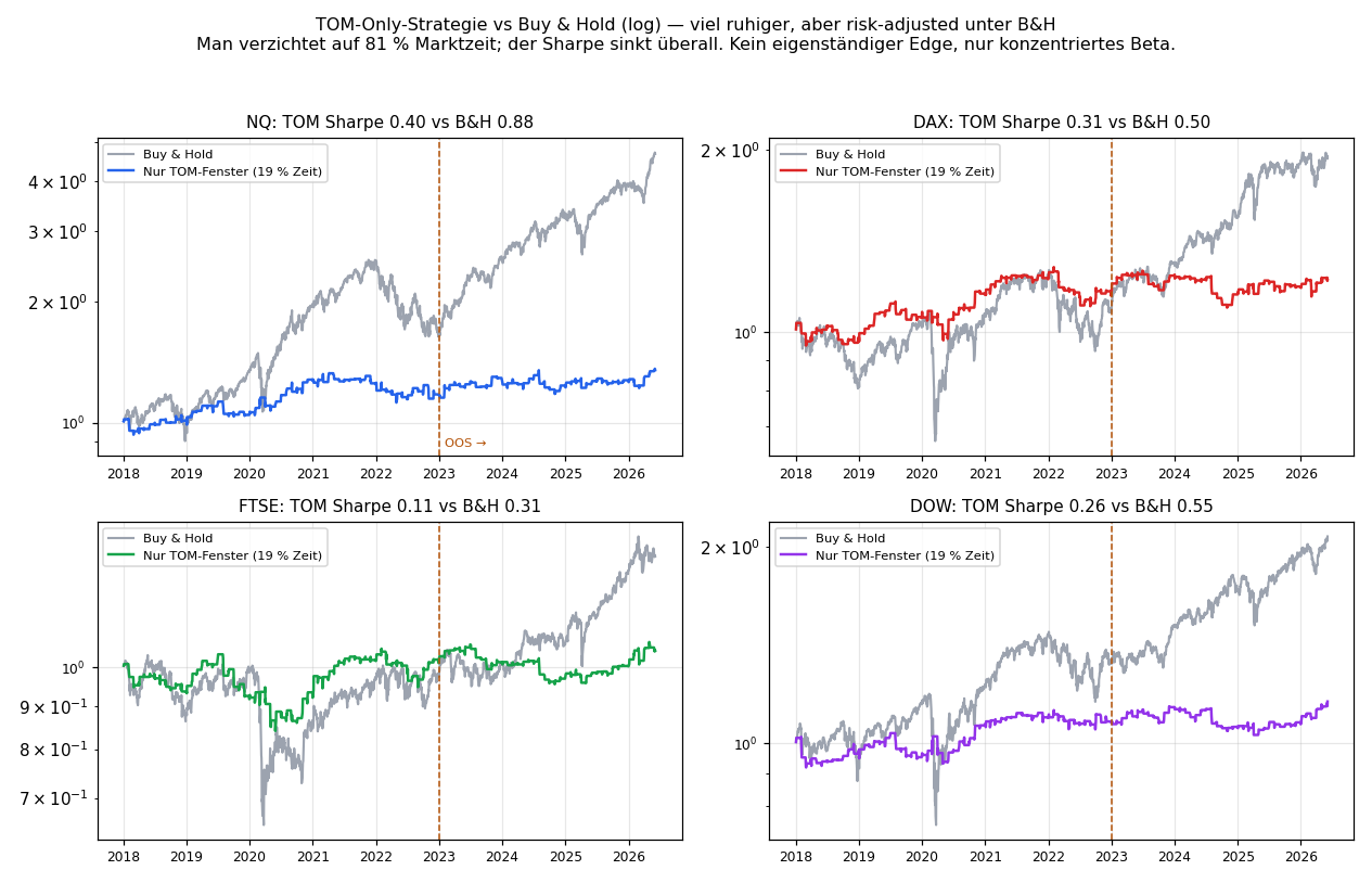
TOM-only is noticeably calmer (half the drawdowns), but the Sharpe is below buy-and-hold on every index. You give up 81% of market time and harvest only concentrated beta — no standalone alpha.
Finding 4 — the rebalancing mechanism
That leaves mechanism (B): is TOM weaker after strong months (rebalancer selling pressure)?
| Index | TOM after UP month | TOM after DOWN month | Supports thesis (B)? |
|---|---|---|---|
| NQ | +0.26% | +0.44% | yes (weak) |
| DAX | +0.22% | +0.14% | no (momentum) |
| FTSE | −0.03% | +0.19% | yes |
| Dow | −0.12% | +0.62% | yes (clear) |
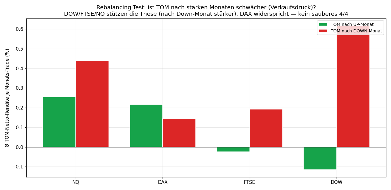
Three of four indices show the expected mean-reversion (TOM stronger after down months), DAX shows the opposite. No clean 4/4 — the two mechanisms appear to overlap differently per market. The effect is clearest on the broadly diversified Dow and weakest on the momentum-driven DAX/NQ — plausible, but far from provable on four markets and ~100 months.
Finding 5 — does it hold out-of-sample?
Unlike the breakout edge (which broke down live after 2024), the TOM concentration persists out-of-sample:
| Index | IS PF / avg-R / Win | OOS PF / avg-R / Win | Trend |
|---|---|---|---|
| NQ | 1.30 / +0.28% / 58% | 1.52 / +0.37% / 64% | stable / slightly up |
| DAX | 1.27 / +0.24% / 59% | 1.15 / +0.12% / 48% | weakened |
| FTSE | 1.06 / +0.05% / 56% | 1.14 / +0.07% / 64% | stable |
| Dow | 1.17 / +0.12% / 58% | 1.26 / +0.14% / 52% | stable |
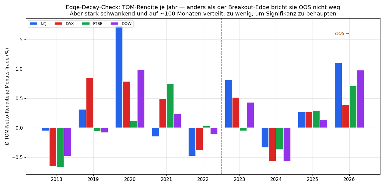
The effect does not vanish — but the PFs are low and spread over only ~40 OOS months. Persistence is not the same as significance.
Finding 6 — the trader frame: is EOM a better trading day?
Findings 1–5 measure accumulated return — the classic academic question "is it a seasonality?". A trader asks something different: is the EOM day a better trading day — bigger, more directional moves, at identifiable times, mechanically capturable? You measure that not via the sum but via the distribution of tradeable daily quantities, conditioned on the event. And here the picture suddenly changes.
EOM days move MORE — 4/4 significant
Mann-Whitney test over the daily distribution (not accumulated):
| Index | Range EOM / Non (p) | |Open−Close| EOM / Non (p) |
|---|---|---|
| NQ | 1.63 / 1.56% (p=0.021) | 0.90 / 0.82% (p=0.008) |
| DAX | 1.30 / 1.27% (p=0.003) | 0.69 / 0.62% (p=0.014) |
| FTSE | 1.08 / 1.04% (p=0.002) | 0.55 / 0.51% (p=0.047) |
| Dow | 1.22 / 1.13% (p=0.001) | 0.65 / 0.57% (p=0.001) |
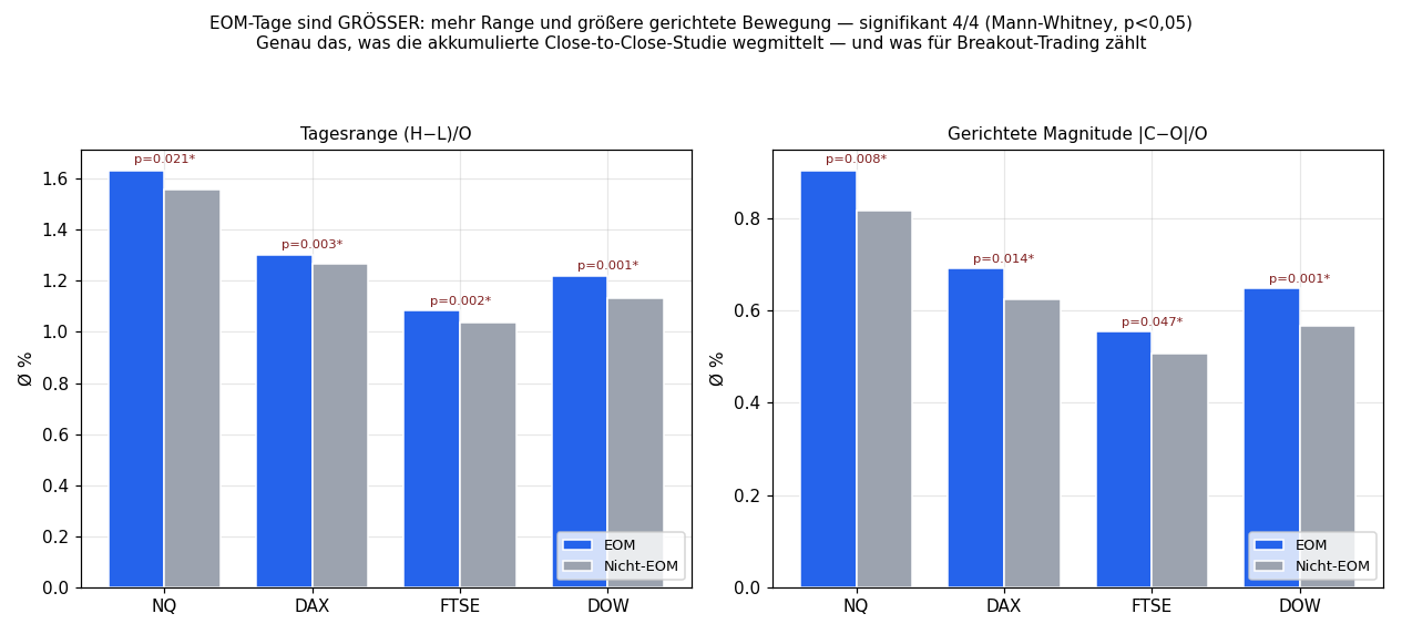
EOM days have larger range and larger directional movement — significant on all four indices. This is exactly what the accumulated close-to-close test averages away — and exactly the property breakout trading likes. (The trend-day rate — close in the top/bottom quartile — is only weakly elevated: DAX/Dow lean "trendier", NQ/FTSE flat. More volatility ≠ automatically more directional persistence.)
At what time? Open and especially the close
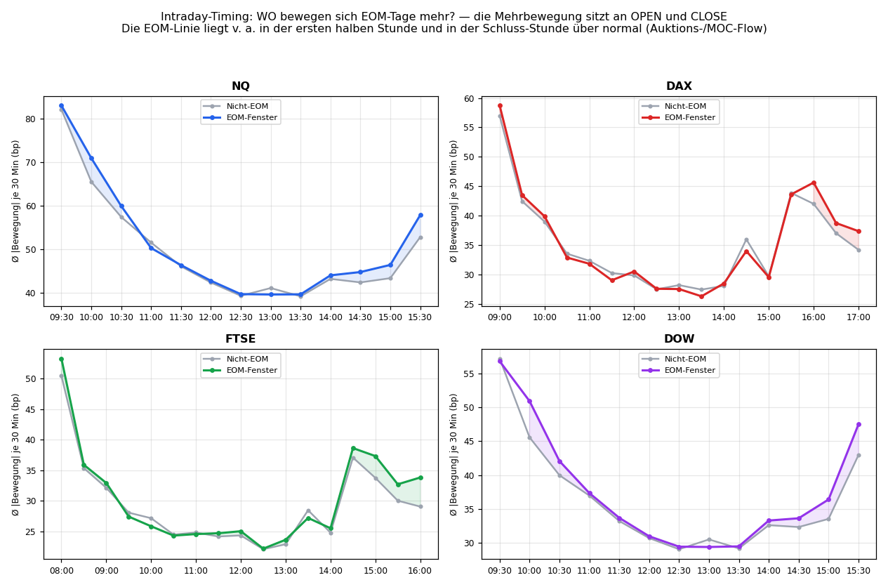
Cut the day into 30-min buckets and the EOM extra movement sits in the first half hour and, above all, in the closing hour — cross-asset (NQ/Dow ~15:00–16:00, DAX 15:30–17:30, FTSE 15:00–16:30). That is mechanism-consistent: rebalancing and MOC orders execute at the close. Precisely the "why" evidence the accumulated test lacked.
Is it exploitable? The breakout test
The same 2nd-candle breakout as in the breakout series, but trades split by EOM vs. non-EOM (net of spread):
| Index | EOM avg-R / PF | Non avg-R / PF | OOS (EOM) |
|---|---|---|---|
| NQ | +0.016 / 1.02 | +0.149 / 1.24 | PF 0.95 ❌ |
| DAX | +0.255 / 1.37 | +0.077 / 1.11 | PF 1.48 ✅ |
| FTSE | +0.076 / 1.10 | −0.125 / 0.84 | PF 1.09 ✅ |
| Dow | +0.229 / 1.37 | +0.049 / 1.08 | PF 0.94 ❌ |
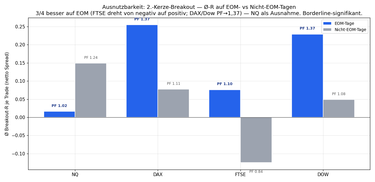
3 of 4 markets trade the breakout better on EOM days: FTSE flips from net-negative (PF 0.84) to positive, DAX/Dow jump to PF 1.37 — and DAX even holds it out-of-sample (PF 1.48). But honestly framed: the difference is only borderline-significant (Welch t 1.25–1.58), NQ contradicts (EOM is worse there), and Dow breaks down OOS. No clean 4/4, no standalone — but a far more useful picture than the accumulated null.
Verdict & the gate
Does the turn-of-the-month effect pass the strict validation gate? No.
| Gate criterion | Result | Passed? |
|---|---|---|
| Cross-asset concentration > 1× | 4/4 | ✅ |
| Significance (Welch t ≥ 1.64) | 0/4 (max 0.40) | ❌ |
| Beats B&H risk-adjusted (Sharpe) | 0/4 | ❌ |
| OOS persistence (PF ≥ 1.0) | 4/4 | ✅ |
| Clean rebalancing mechanism (4/4) | 3/4 | ❌ |
Two "yes" are not enough — an edge must clear the hard hurdles (significance, beating B&H), not just the soft ones. As a standalone, accumulated return effect, the turn-of-the-month effect is therefore rejected. But the trader frame (Finding 6) delivers the actually usable part: EOM days are 4/4-significantly larger movement days, with the extra movement at open and close — and therefore more breakout-friendly on 3/4 markets (DAX OOS-stable).
How do you use this honestly? Not as a strategy but as a conditioning signal — exactly method #3 of the methodology (risk/size adjustment instead of a hard filter): on EOM days run breakout risk higher, on normal days lower; trade a borderline market like FTSE only on EOM days mechanically. This is not a "why-effect that beats beta" — over very long horizons (Lakonishok-Smidt, 90 years of Dow) the return effect is documented, but our 8.5-year window is too short to confirm it. The tradeable part is the volatility concentration, not the direction — and that one is real, borderline-significant, and belongs in risk management, never as a standalone money machine.
Limitations & the methodological lesson
- Sample length. ~100 month boundaries are few for a monthly effect. The literature works with decades; our power is correspondingly low.
- Correlated markets. Four equity indices are not four independent samples — the 4/4 rule is weaker here than for uncorrelated assets. That is exactly why the pooled test (which also fails).
- Beta confusion. The concentration largely measures the upward drift within a time window, not alpha. The B&H comparison exposes this.
- Data definition. Cash close-to-close including the overnight gap; a different close definition could shift the numbers slightly.
This run is the counterpart to the breakout series: there, patterns failed without a reason; here, a well-reasoned mechanism fails the gate anyway. Both paths lead to the same discipline and the same insight: a convincing why does not replace a significance test, and a pretty aggregate number is not an edge. The most honest result of a research program is often a cleanly documented "does not work as a standalone." How the full workflow is built is described in the methodology reference.
📄 Full study as PDF · See also: 2nd opening candle · validation gate